Large language models can write sonnets, fix code and explain photosynthesis in the voice of a pirate. They are one of the most remarkable things computer science has produced, and this essay is not here to argue otherwise.
It is here to stick up for an older, quieter idea that does not get as much attention as it deserves: convexity. Convex optimisation will not write you a sonnet. But when there is not much data, when someone needs to know why, when the answer is needed in a few milliseconds, or when every experiment costs real money, it is often the best tool you can pick up. And as we will see, it works very well alongside the big models.
The marble and the bowl
Picture a marble dropped into a smooth bowl. Wherever you let go of it, it rolls down and settles at the same spot: the bottom. There is only one bottom, and the marble cannot miss it.
Now picture dropping the same marble onto a mountain range in thick fog. It rolls downhill, but “downhill” might lead into a small valley halfway up a mountain. The marble stops there. It has no way of knowing that a much deeper valley lies two ridges over.
These are the two kinds of problems this essay is about.
- A convex problem is a bowl. Any way downhill leads to the best answer, and once you are at the bottom you can prove that you are there.
- A non-convex problem is a mountain range. You can usually find a good valley, but you can rarely be sure it is the best one.
Training a neural network is a hike through a mountain range with billions of directions instead of two. It works astonishingly well, which is one of the pleasant surprises of the last fifteen years. But it needs huge amounts of data and computing power, and run it twice from different starting points and you will usually land in two different valleys.
Real problems also come with rules. A budget cannot be overspent. A battery cannot hold more charge than it has room for. A robot arm cannot push harder than its motor allows. You can think of a rule as a fence that the marble is not allowed to cross. As long as the fenced-in area has no dents (if you can stand at any two allowed points and walk in a straight line between them without leaving the area), the problem is still a bowl. There is still exactly one lowest point inside the fence1.
1 Strictly speaking, one lowest value. A bowl with a flat bottom has many equally good lowest points, and they all count as the answer.
- Objective: the thing you want to make as small as possible (cost, error, wasted energy). It is the height of the bowl.
- Constraint: a rule the answer must obey. One of the fences.
- Linear program (LP) and quadratic program (QP): two of the simplest and most common kinds of bowl.
- Dual or shadow price: how much better the answer would get if a particular fence were moved back a little. More on these soon. They are the hero of the interpretability section.
Two players and a saddle
How do you actually find the bottom of a fenced-in bowl? One elegant method turns the problem into a game between two players.
The first player, the builder, tries to make the objective as small as possible. The second player, the referee, watches the fences. Every time the builder strays past one, the referee raises the fine for that fence. Every time the builder stays comfortably inside, the referee eases off. The two take turns, and the game ends when neither can do any better.
The point where they settle is called a saddle point. It is named after a horse’s saddle, which is a low point if you look from front to back and a high point if you look from side to side. The builder ends up with the best allowed answer. The referee ends up with a fine for every fence: the shadow prices. Keep those fines in mind. They turn out to be very useful.
A general convex solver lets you describe your bowl and your fences as ordinary code and leaves everything else to the computer. You do not derive the slopes by hand, because automatic differentiation (the same trick that trains neural networks) works them out. That matters more than it sounds, and we will come back to it at the end.
1. When data is scarce
Foundation models learn from trillions of words. Plenty of important problems come with a spreadsheet of two hundred rows.
With two hundred rows, a model with a billion adjustable knobs has nothing to anchor it. It will memorise the spreadsheet and learn very little. A convex model has far fewer knobs, and its bowl shape means those knobs settle in one sensible place rather than wandering off to fit the noise.
Here is a small experiment. Make up some data with fifty possible causes, of which only five really matter, add some noise, and keep just two hundred examples. A classic convex method called the lasso looks for an answer that fits the data and uses as few causes as possible. It reliably sets most of the fifty weights to exactly zero and points to the handful that matter2. It is like a detective who explains the crime with the fewest suspects.
2 Fifty correlated features, five of them real, two hundred samples. The lasso is a bowl once each weight is split into a positive and a negative part, which leaves only “must be at least zero” fences.
There is a second, bigger advantage. When data is scarce, knowledge is precious, and convex problems let you write knowledge down directly as constraints instead of hoping the data will teach it:
- “This should only ever go up.” Bigger houses cost more. Higher doses do not make a medicine less effective. One line of code that says “each value is at most the next one” turns a wobbly, noisy curve into a clean staircase that only climbs3.
- “Physics is not optional.” If you are tracking a moving vehicle, its position next second depends on its position and speed now. Write that down as an equality constraint and the model cannot propose a car that teleports.
- “Some of the data is rubbish.” Swap the usual squared error for a gentler penalty (the Huber function) that grows only in a straight line for large mistakes. Now a sensor that occasionally shouts nonsense cannot drag the answer away. Even when a fifth of the readings are wild outliers, the estimated path stays on the road4.
3 This is isotonic regression, and its whole definition fits in a single lambda. See the code sketch near the end.
4 A robust Kalman smoother over a thousand time steps. The ordinary least-squares smoother gets pulled off course by the outliers, while the Huber version calmly ignores them.
Each of those rules is worth a great many training examples, and none of them needs a GPU cluster to learn.
2. When you need to know why
Ask a large language model why it gave an answer and it will give you a fluent, plausible explanation. Whether that explanation describes what really happened inside the model is a hard open research question.
Convex models tend to explain themselves in three more concrete ways.
The weights mean something. A convex model often has a small number of weights attached to things a person can name. A search ranker might use seventeen features such as “how many of the query’s words appear in the title” or “how long is this document”. Each one gets one weight, and you can read the list like a recipe. The lasso goes further and hands you a short list of the causes it thinks matter, with everything else set to zero.
The referee’s fines are explanations. Remember the saddle game? The fine on each fence tells you how much the objective would improve if that fence moved back a little. Economists call this a shadow price, and it answers questions people actually ask:
- A shipping company limits its carbon emissions. The fine on the emissions fence is, in effect, the carbon price the company is paying, in dollars per tonne, even though nobody wrote that price down5.
- An investor caps how risky a portfolio may be. The fine on the risk fence says how much extra return one more unit of risk would buy6.
- A lender requires that its loan-approval model treat two groups of applicants fairly. The fine on the fairness fence is the price of fairness: how much the model’s fit to past decisions suffers for each step towards equal treatment.
5 The fines on the demand constraints give each market’s marginal cost of supply in the same way.
6 Sweep the risk limit and that fine is the slope of the efficient frontier, read directly off the solver rather than estimated.
That last example has a twist worth telling. Suppose the lender’s past decisions were unfair, and it tries to fix this by simply hiding which group each applicant belongs to. It does not work. Other details, like a postcode, quietly carry the same information, and the model rediscovers the old bias. A constraint is more honest. It says exactly what “fair” should mean, enforces it, and the shadow price states plainly what that choice costs. In that made-up world the fair model even agrees better with what applicants deserved, because the bias was in the old labels, not in the people.
The solver can prove it is finished. For a convex problem, the builder’s answer and the referee’s fines together give a number called the duality gap. When the gap is small, the answer is provably close to the best possible one, no matter how the solver got there. It is a homework answer that comes with its own marking scheme. Few other corners of machine learning can offer that.
3. When the answer is needed now
A large language model performs billions of calculations for every word it writes. For a chatbot that is fine, since people read slowly. For a robot arm that must react within a few milliseconds, or a power grid balancing itself second by second, it is far too slow.
Convex problems used for control are often tiny. Picture a chain of four blocks joined by springs, with a wall at each end and three small motors pushing neighbouring blocks apart. Every half a second a controller looks at where the blocks are, plans the next few seconds of motor pushes, applies the first one, then plans again. This is called model predictive control. Each plan is a quadratic program with about a hundred variables. A good solver finishes it in a fraction of a millisecond.
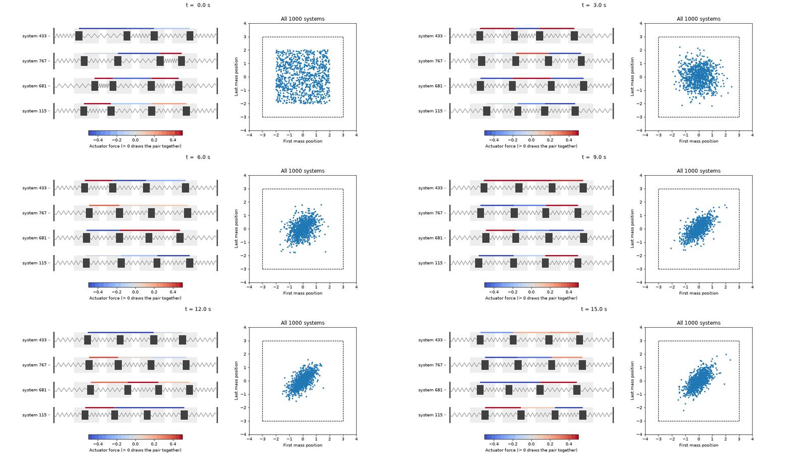
Now make it a fleet of a thousand such systems: a thousand delivery drones, say, or a thousand batteries on a grid. Their problems all have the same shape and differ only in their current state. A batched convex solver on a GPU handles all thousand at once, in lockstep, and each plan starts from the previous half-second’s plan shifted forward, which is an excellent first guess. On one laptop GPU this works out to about one fortieth of the time per problem of a well-tuned CPU solver working through the fleet one problem at a time.
There is an honest caveat. For a single system on its own, the CPU solver wins, because a lone tiny problem leaves a GPU sitting idle. A GPU is a bus, not a sports car. It shines when there are lots of passengers going the same way.
Two more things make convex solvers a comfortable fit for deadlines:
- They keep their promises along the way. A solver can be built so that every intermediate answer already respects the hard limits, such as “the motor can’t push harder than this”. If the deadline arrives before the solver has fully converged, the plan you take is slightly less than perfect, but it is not illegal.
- The trained model is often tiny. A linear search ranker scores a document with seventeen multiplications and some additions. That is cheap enough to run on every candidate document without anyone noticing.
4. When every experiment costs money
Training a large neural network involves dozens of settings: the learning rate, how it changes over time, the batch size, the random seed, and many more. Getting them wrong can quietly ruin a training run that cost a great deal to do. Teams search over these settings by training many slightly different models, and each one is a full, expensive run.
Convex problems remove most of that search, for a simple reason. The answer depends only on the bowl, not on how you rolled the marble. Different starting points, different step sizes and different random seeds all lead to the same bottom. The only settings left are the ones that mean something: how strongly to favour simple models, how fair the lender must be, how much risk the investor will accept.
Better still, those meaningful settings are cheap to explore:
- Solve many bowls at once. Problems with the same shape can be stacked and solved together. A lasso can be solved for a whole range of simplicity settings in one batched call. The lender’s fairness trade-off can be traced across forty thresholds in a single solve, giving a curve of accuracy against fairness and the price of fairness at every point along it. A search ranker’s regularisation path of eleven problems takes about three seconds on a laptop GPU.
- Start from the last answer. Neighbouring settings have neighbouring answers, so each solve can warm-start from the one before. Tracing out an investor’s whole menu of risk-versus-return choices becomes a quick walk rather than a series of cold starts.
- Follow the slope instead of searching a grid. Because the bottom of the bowl moves smoothly as you change a setting, you can work out which way to change it, using the same calculus trick that trains neural networks. Give each of the lasso’s fifty features its own penalty, and a grid search over fifty settings becomes hopeless, since even two values each would mean more than a thousand trillion combinations. Gradient descent tunes all fifty at roughly the cost of tuning one, and brings the error on fresh test data down to the level of the noise itself, which is as good as any model can do.
The same trick works one level up. To decide how big a home battery to buy, you need to know how cleverly it would be run, and running it well for a day is itself a small linear program. Solve a month of such days in one batch, ask how the total cost changes as the battery grows, and roll downhill on the battery’s size7. The convex solver becomes a building block inside a larger optimisation.
7 Thirty-two scenario days, each with its own prices, demand and sunshine, and forty steps of gradient descent on the battery’s size. The sizing problem itself is not a bowl, because big batteries are cheaper per kilowatt-hour, which is exactly why it gets split up this way.
And yet it performs surprisingly well
All of this would be a nice story if convex methods were safe, cheap and a little bit rubbish. They are not.
Take search, which matters to anyone building a chatbot that looks things up before it answers. One common test asks a system to find the scientific papers that support or refute a claim, and scores it out of 1 on how good its top ten results are. Here is how some approaches fare on that test:
| Approach | Score (out of 1) |
|---|---|
| Keyword matching (BM25) | 0.681 |
| A small neural embedding model | 0.720 |
| Keywords and embeddings blended together | 0.731 |
| Convex reranker using all of the above as features | 0.770 |
The winner is a ranking support vector machine: a convex quadratic program with seventeen weights. It adds about four points over the blended system, and a statistical check puts that gain between two and six points8. Every training run gives the same answer, the solver certifies it, and the seventeen weights can be printed on a postcard.
8 Test nDCG@10 on SciFact, with a 95% bootstrap interval of +0.021 to +0.060 over reciprocal rank fusion.
Look closely at that table, though, because it holds the most important lesson in this essay. One of the reranker’s seventeen features is the neural embedding model. Without the embedding features, a keyword-only version of the same reranker scores 0.724. The convex model did not beat the neural network. It used the neural network, and did better than either could alone.
Friends, not rivals
That pattern repeats, and it suggests a sensible division of labour.
- Foundation models make features, convex models make decisions. A neural network turns messy text, images or sound into useful numbers. A convex model combines those numbers under rules you can state and audit.
- Convex layers act as guardrails. A neural network proposes, and a convex problem projects that proposal onto the set of things that are allowed: within budget, within physical limits, within the fairness rules.
- Language models can write the bowl. Describing a problem in a modelling language is something language models are increasingly good at. The convex solver then supplies what the language model cannot: a certified optimum and a set of shadow prices that explain it. The language model writes the essay and the solver checks the arithmetic.
There are also places where convexity is simply the wrong tool. Recognising a cat in a photo, translating a poem, holding a conversation: nobody knows how to write these down as bowls, and the mountain-range methods are the right answer. The trick is to notice when part of your problem is a bowl, and to treat that part accordingly.
Why general matters
For decades, convex optimisation came in specialised boxes: one solver for linear programs, another for quadratic programs, a third for this particular statistics problem. Each had its own input format and its own quirks. Using one meant first translating your problem into the box’s language, which was often the hardest part.
A general solver turns this around. You write the objective and the rules as ordinary code, and the solver works out the rest. Here is the whole definition of a monotone curve fit:
import jax.numpy as jnp
import jaddle.jaddle_convex as jc

y = jnp.linspace(-1.0, 1.0, 100) ** 3   # data to fit

cp = jc.JaddleCP(
    num_variables=100,
    objective=lambda p: jnp.sum((p - y) ** 2),   # stay close to the data
    constraints_eq=lambda p: jnp.zeros(0),       # no equality rules
    constraints_ineq=lambda p: p[:-1] - p[1:],   # each value <= the next
    lower_bounds=-jnp.ones(100),
    upper_bounds=jnp.ones(100),
)

result = jc.solve(cp)
The same machinery then handles a search ranker, a fair lender, a thousand-strong fleet of controllers, a log-optimal investment portfolio or a noisy-channel capacity calculation, on a laptop CPU or a GPU, without a new solver for each. Because it is built on the same tools as modern deep learning, it can be batched, differentiated and dropped into a larger model like any other layer.
When the cost of trying a convex formulation falls to a few lines of code, it stops being the thing you reach for once everything else has failed and becomes the first thing you try. That is the real argument for a general solver. Convexity was never about the mathematics being pretty (though it is). It is about making the guarantees, explanations, speed and cheap experiments easy enough to use every day.
In short
Foundation models are superb mountaineers, and the world is full of mountains. But it is also full of bowls: budgets, schedules, controllers, rankers, fair classifiers, portfolios. When you meet one, you are in luck. You can find the very bottom, prove that you have found it, explain why it is there, and do it again for a thousand slightly different bowls before lunch.
So the next time a problem lands on your desk, before reaching for the biggest model you can find, it is worth asking a small question first:
Is this a bowl?