Imagine you’ve been put in charge of the smoke detectors for an entire country. There’s one catch: you only get 50 of them. Where do you put them?
That’s not just a thought experiment. The US Environmental Protection Agency (EPA) runs about a thousand monitors that measure PM2.5: specks of dust, soot and smoke so small that about thirty of them side by side would match the width of a human hair. They’re small enough to get deep into your lungs, so knowing how much is in the air each day matters.
Every five years, each US state has to review its monitoring network. Is it still doing its job? Do we need more monitors? Could a few be retired? Behind all of that sits one question:
If I can afford
kmonitors, whichkspots tell me the most about the air in all the places where I don’t have a monitor?
I built an example for Jaddle, an optimisation library I work on, that answers this question with two years of real EPA data. Here’s how it works, no PhD needed.
Why this is harder than it looks
After some tidying up (keeping sites that report reliably in both 2023 and 2024), we have 705 sites. I set aside a random third of them, 235 sites, as targets: places where we want to know the air quality but won’t put a monitor. The other 470 are candidates.
How many ways are there to pick 50 sites from 470? About 10^68. That’s a 1 followed by 68 zeros, more than the number of atoms that make up the Earth (a mere 10^50 or so). Even checking a billion networks a second, you’d still be going long after the Sun burns out.
So we need to be clever.
Step 1: Learn how the air behaves
Air pollution doesn’t happen site by site. A weather system parks over the Midwest, or wildfire smoke drifts in from Canada (as it did across the Northeast in June 2023), and whole regions go up and down together.
That’s useful. If you know how a few places are doing, you can make a good guess about their neighbours, a bit like guessing the score of a football match from the crowd noise outside the stadium.
Using the 2023 data, the model learns 20 regional patterns (weather systems, smoke plumes, the seasons) and how strongly each site follows each one. Those 20 patterns explain about 76% of the day-to-day ups and downs. The rest is local: a busy road, a neighbour’s barbecue, a wobbly sensor.
Once we have that model, we can score any network: how much of the regional pattern at the targets does it leave unexplained? Lower is better.
Step 2: Swap the light switch for a dimmer
Each candidate site is like a light switch: monitor on or off. All those on/off choices are what make the problem so huge.
So we cheat, temporarily. We replace every switch with a dimmer, so a site can have 0.4 of a monitor, or 0.93 of a monitor. The rule is that the dimmers must add up to 50.
That sounds silly, but it turns a bumpy, impossible search into a smooth convex problem. Picture a bowl: wherever you drop a marble, it rolls to the same lowest point. Jaddle’s convex solver found the bottom of this bowl in 36 steps, about 3 seconds.
Then we turn the dimmers back into switches. We keep the 50 brightest sites, then try swapping a chosen site for an unchosen one, keeping any swap that helps. After just 5 swaps nothing else improves.
Step 3: Get a receipt
This is my favourite part.
The dimmer version of the problem has more freedom than the real one: every real network is just a dimmer setting where each dial happens to be at 0 or 1. So the best dimmer answer is a floor. No real network of 50 monitors can ever do better than it.
Our network lands within 1.3% of that floor. So without checking all 10^68 options, we can say with confidence that no 50-monitor network beats ours by more than about 1.3% (as judged by the model).
Most methods hand you an answer. This one hands you an answer and a receipt.
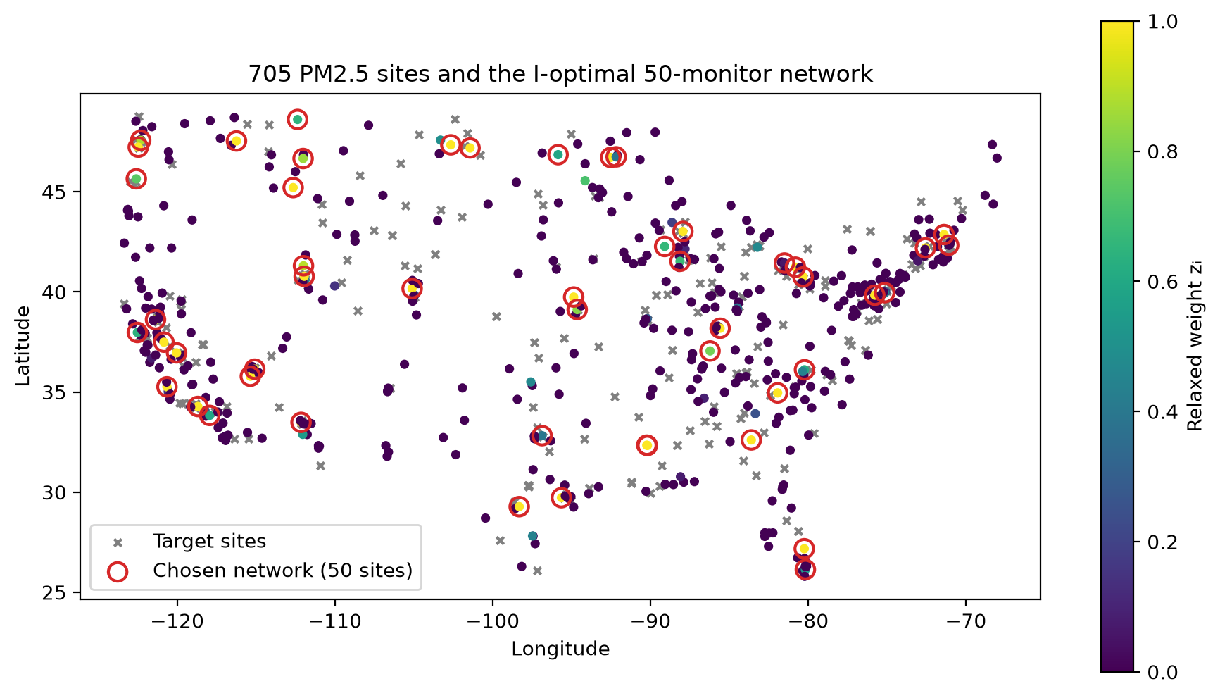
A few things jump out of the map:
- The chosen sites aren’t evenly spaced. There are clusters along the West Coast and in the Northeast, where lots of people (and lots of target sites) live.
- Big empty areas still get a monitor or two. One well-placed sensor can “speak for” a whole region that moves together.
- Most dimmers ended up fully on or fully off. Only 47 of the 470 were in between, so turning the dimmers back into switches was easy.
Did it actually work? The 2024 exam
A model that’s only tested on the data it learned from is like a student marking their own homework. So the real test uses 2024, a year the model never saw.
For each network, we predicted the daily PM2.5 at all 235 target sites from that day’s readings at the 50 monitors, then measured the typical error:
| 50 monitors, placed by… | Typical error in 2024 (µg/m³) |
|---|---|
| Nobody (just use last year’s average) | 5.21 |
| Spreading them evenly over the map | 4.16 |
| Picking at random (average of 20 tries) | 4.04 |
| Greedy: add the most helpful site, one at a time | 3.70 |
| Optimised design (this article) | 3.71 |
The optimised network cuts the error by about 8% compared with random picks, on data it had never seen.
Two things surprised me:
- Spreading monitors evenly does worse than random. It feels fair, but it puts sensors in big, empty, mostly clean areas. The largest errors come from smoggy days in crowded places, and an even spread under-covers those.
- The simple “greedy” method is just as good here. I’ll be honest about that. Greedy is a strong, well-known approach. What it can’t give you is the receipt. Only the dimmer trick can tell you that nothing out there does much better.
How many monitors is enough?
Fifty was an arbitrary choice, so I asked Jaddle to solve the problem for 16 different budgets, from 5 to 150 monitors, in one batched call (using JAX’s vmap, which runs many copies of the solver side by side).
The headline:
- About 35 well-placed monitors predict as well as 150 randomly placed ones. Placement matters more than quantity.
- Returns shrink fast. The 150th monitor is worth roughly a fiftieth of the 16th. For a state deciding which monitors to retire, that curve shows where cutting starts to really hurt.
- The receipt gets better as the budget grows: within 5% of the floor from about 24 monitors, and within 0.1% at 150.
Bonus: which monitor deserves an upgrade?
The solver can also say how much better the best possible network would get if any single site had a less noisy sensor (for example, by installing a second instrument next to the first). One calculation covers all 705 sites at once.
The top of the list: Tacoma (South 36th St), Washington, followed by sites in California, Colorado, Idaho and Nevada. So the same tool that picks locations also points to where an equipment upgrade would help most.
The takeaways
- Many “choose the best few” problems are secretly huge. Picking 50 from 470 has more options than there are atoms in the Earth.
- Relaxing the rules helps you solve the strict version. Swapping switches for dimmers turns an impossible search into a 3-second solve.
- A good answer with a guarantee beats a good answer alone. The relaxation doesn’t just find a strong network; it proves there isn’t a much better one.
- Test on data the model hasn’t seen. The improvement held up in 2024, though it was smaller than the model predicted, because some pollution is just local and no network can see it coming.
Try it yourself
The full example, from downloading the EPA data to drawing the map, is examples/cp/monitor_network_design.py in the Jaddle repository. It runs in a few minutes and uses only public data.
If you work on sensor placement, experimental design or any other “where do I put my limited stuff?” problem, I’d love to hear how you approach it.